2. Reference matching tutorial#
In this tutorial you will learn how to map query to reference scATAC-seq dataset using cisTopic model of the data. This pipeline is a slightly modified version of hnoca-tools, which was developed for matching scRNA-seq data.
Prepare reference#
import os

os.environ["SCIPY_ARRAY_API"] = "1"

# Import required packages
import numpy as np
import pandas as pd
import scanpy as sc
from scarches.models.scpoli import scPoli  # Import scPoli directly
from atac_mapper.reference_mapping.mapping_atac import AtlasMapper
import scarches
import matplotlib.pyplot as plt
import seaborn as sns

%matplotlib inline
Now that we’ve reloaded the module, we can proceed with the rest of the notebook. Remember to rerun this reload cell whenever you make changes to your package files.
adata_ref = sc.read_h5ad("../../../../test_data_atac_mapper/reference_adata_ZH.h5ad")
adata_ref
AnnData object with n_obs × n_vars = 99732 × 175
    obs: 'Transcriptome', 'Strain', 'Sex', 'Method', 'Editat', 'Donor', 'NPeaks', 'is__cell_barcode', 'Chemistry', 'Ageunit', 'sample_id', 'DoubletFinderScore', 'duplicate', 'Neuronprop', 'Plugdate', 'Analysis', 'CellID', 'Shortname', 'Splits', 'peak_region_fragments', 'cisTopic_log_nr_frag', 'regions', 'peak_region_cutsites', 'Datecaptured', 'mitochondrial', 'Clusters_main', 'cisTopic_nr_frag', 'Agetext', 'Project', 'ClusterName', 'Editby', 'All_fc_analysis_id', 'TSS_fragments', 'Tissue', 'chimeric', 'SubClusters', 'Sampleok', 'Celltype', 'Cellclass', 'batch', 'conditions_combined', 'presence_max_MBO', 'isDA'
    var: 'highly_variable', 'means', 'dispersions', 'dispersions_norm', 'highly_variable_nbatches', 'highly_variable_intersection', 'mean', 'std'
    uns: 'Agetext_colors', 'Cellclass_colors', 'Celltype_colors', 'Donor_colors', 'Shortname_colors', 'Tissue_colors', 'harmony', 'hvg', 'isDA_colors', 'neighbors', 'pca', 'scpoli', 'umap'
    obsm: 'X_pca', 'X_pca_harmony', 'X_scpoli', 'X_tsne', 'X_umap', 'X_umap_bbknn', 'X_umap_harmony', 'X_umap_raw', 'X_umap_scpoli'
    varm: 'PCs'
    layers: 'Raw_topic', 'scaled'
    obsp: 'connectivities', 'distances', 'harmony_connectivities', 'harmony_distances', 'scpoli_connectivities', 'scpoli_distances'
adata_ref.X = adata_ref.layers["scaled"].copy() # set scaled topic distribution as X
Let’s train reference scPoli model. (Could be done on CPU, if no GPU are available, just takes more time).
adata_ref.obs["batch"] = adata_ref.obs["Donor"].copy()  # set Donor as batch
scpoli_model = scarches.models.scpoli.scPoli(
    adata=adata_ref,
    condition_keys="batch",
    cell_type_keys=["Cellclass", "Celltype"],
    unknown_ct_names=["Unknown"],
    hidden_layer_sizes=[128],
    latent_dim=20,
    embedding_dims=5,
    recon_loss="mse",  # needed for continious data as we have in topics
)

early_stopping_kwargs = {
    "early_stopping_metric": "val_prototype_loss",
    "mode": "min",
    "threshold": 0,
    "patience": 20,
    "reduce_lr": True,
    "lr_patience": 13,
    "lr_factor": 0.1,
}
Embedding dictionary:
 	Num conditions: [26]
 	Embedding dim: [5]
Encoder Architecture:
	Input Layer in, out and cond: 175 128 5
	Mean/Var Layer in/out: 128 20
Decoder Architecture:
	First Layer in, out and cond:  20 128 5
	Output Layer in/out:  128 175
scpoli_model.train(
    n_epochs=50,
    pretraining_epochs=35,
    early_stopping_kwargs=early_stopping_kwargs,
    eta=10,
    alpha_epoch_anneal=20,
    batch_size=4096,
)
Initializing dataloaders
Starting training
 |██████████████------| 70.0%  - val_loss:   93.62 - val_cvae_loss:   93.62
Initializing unlabeled prototypes with Leiden with an unknown number of  clusters.
Clustering succesful. Found 33 clusters.
 |████████████████████| 100.0%  - val_loss:  242.95 - val_cvae_loss:  163.74 - val_prototype_loss:   79.21 - val_unlabeled_loss:    2.10 - val_labeled_loss:    7.92
Let’s save the model and get latent embeddings
scpoli_model.save("scpoli_reference_model", overwrite=True)

adata_ref.obsm["X_scpoli"] = scpoli_model.get_latent(adata_ref, mean=True)
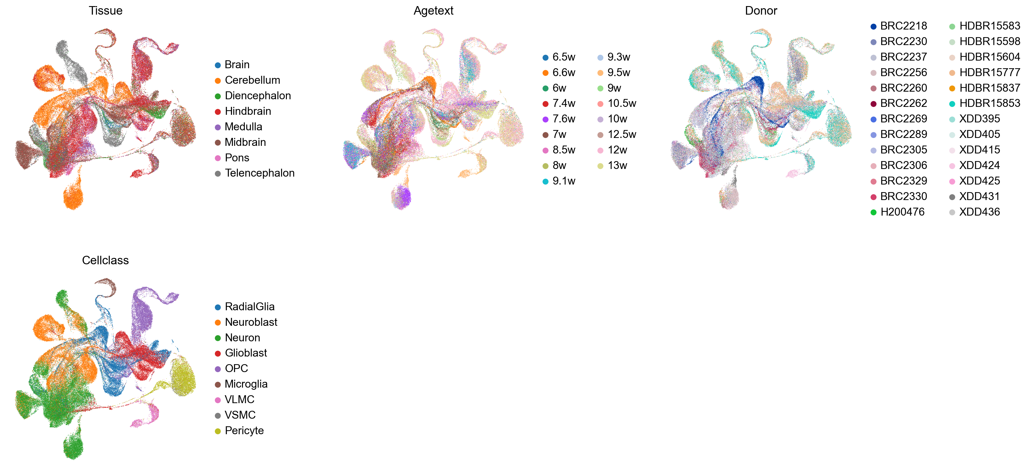
Let’s visualise the latent space embedding of the reference data
sc.pp.neighbors(adata_ref, use_rep="X_scpoli", key_added="scpoli")
sc.tl.umap(adata_ref, neighbors_key="scpoli")
adata_ref.obsm["X_umap_scpoli"] = adata_ref.obsm["X_umap"].copy()
with plt.rc_context({"figure.figsize": (4, 4.5)}):
    sc.pl.embedding(
        adata_ref,
        basis="X_umap_scpoli",
        color=["Tissue", "Agetext", "Donor", "Cellclass"],
        frameon=False,
        ncols=3,
        wspace=0.5,
    )
Map query data using scPoli model#
# Load pre-trained scPoli model
ref_model = scPoli.load("scpoli_reference_model", adata=adata_ref)

# Initialize mapper with the loaded model
mapper = AtlasMapper(ref_model)
AnnData object with n_obs × n_vars = 99732 × 175
    obs: 'Transcriptome', 'Strain', 'Sex', 'Method', 'Editat', 'Donor', 'NPeaks', 'is__cell_barcode', 'Chemistry', 'Ageunit', 'sample_id', 'DoubletFinderScore', 'duplicate', 'Neuronprop', 'Plugdate', 'Analysis', 'CellID', 'Shortname', 'Splits', 'peak_region_fragments', 'cisTopic_log_nr_frag', 'regions', 'peak_region_cutsites', 'Datecaptured', 'mitochondrial', 'Clusters_main', 'cisTopic_nr_frag', 'Agetext', 'Project', 'ClusterName', 'Editby', 'All_fc_analysis_id', 'TSS_fragments', 'Tissue', 'chimeric', 'SubClusters', 'Sampleok', 'Celltype', 'Cellclass', 'batch', 'conditions_combined', 'presence_max_MBO', 'isDA'
    var: 'highly_variable', 'means', 'dispersions', 'dispersions_norm', 'highly_variable_nbatches', 'highly_variable_intersection', 'mean', 'std'
    uns: 'Agetext_colors', 'Cellclass_colors', 'Celltype_colors', 'Donor_colors', 'Shortname_colors', 'Tissue_colors', 'harmony', 'hvg', 'isDA_colors', 'neighbors', 'pca', 'scpoli', 'umap'
    obsm: 'X_pca', 'X_pca_harmony', 'X_scpoli', 'X_tsne', 'X_umap', 'X_umap_bbknn', 'X_umap_harmony', 'X_umap_raw', 'X_umap_scpoli'
    varm: 'PCs'
    layers: 'Raw_topic', 'scaled'
    obsp: 'connectivities', 'distances', 'harmony_connectivities', 'harmony_distances', 'scpoli_connectivities', 'scpoli_distances'
Embedding dictionary:
 	Num conditions: [26]
 	Embedding dim: [5]
Encoder Architecture:
	Input Layer in, out and cond: 175 128 5
	Mean/Var Layer in/out: 128 20
Decoder Architecture:
	First Layer in, out and cond:  20 128 5
	Output Layer in/out:  128 175
Load Query Dataset#
Now we’ll load the query dataset (atlas_500_test.h5ad) that we want to map to our reference.
# Load query dataset
adata_query = sc.read_h5ad("../../../../test_data_atac_mapper/atlas_aftersymphony_cistopic_ZH.h5ad")
adata_query
AnnData object with n_obs × n_vars = 104452 × 175
    obs: 'orig.ident', 'nCount_RNA', 'nFeature_RNA', 'nCount_ATAC', 'nFeature_ATAC', 'experiment', 'done_by', 'sample', 'age', 'protocol', 'nucleosome_signal', 'nucleosome_percentile', 'TSS.enrichment', 'TSS.percentile', 'percent.mt', 'percent.rp', 'S.Score', 'G2M.Score', 'Phase', 'RNA.weight', 'ATAC.weight', 'RNA_snn_res.0.5', 'nCount_ATAC_main', 'nFeature_ATAC_main', 'score_NPC', 'score_neuron', 'neuron_NPC', 'annot_revised', 'seurat_clusters', 'Consensus_line', 'Line_quality', 'final_region2', 'annot_level_1', 'annot_level_2', 'annot_level_3', 'annot_level_4', 'gaus_scanvi_q2r', 'cell_types_NA_24', 'region_NA_24', 'fullname_NA_24', 'wsnn_res.20', 'Celltype', 'regions', 'symphony_per_cell_dist', 'Cellclass_wknn', 'Celltype_wknn', 'Agetext_wknn', 'Tissue_wknn', 'pearsonr_topics_Mannens_matched', 'euclidean_topics_Mannens_matched'
    uns: 'Cellclass_wknn_colors', 'Celltype_colors', 'Celltype_wknn_colors', 'Consensus_line_colors', 'Tissue_wknn_colors', 'fullname_NA_24_colors', 'protocol_colors', 'regions_colors', 'scpoli_mannens', 'umap'
    obsm: 'X_pca_harmony', 'X_pca_harmony_symphony_R', 'X_pca_reference', 'X_scpoli_Mannens', 'X_tsne', 'X_umap', 'X_umap_scpoli_Mannens', 'X_umap_symphony_Mannens'
    layers: 'scaled2Mannens'
    obsp: 'scpoli_mannens_connectivities', 'scpoli_mannens_distances'
Scale query to reference#
adata_query.layers["Raw_topic"] = adata_query.X.copy()
adata_query.X = np.apply_along_axis(lambda x: (x - adata_ref.var["mean"]) / adata_ref.var["std"], 1, adata_query.X)
adata_query.X[adata_query.X > 10] = 10
adata_query.layers["scale2ref"] = adata_query.X.copy()
Set Up Reference Mapping#
We’ll now set up the reference mapping using the AtlasMapper with the loaded reference model. The mapper will help us project the query data onto the reference space.
# Map query data to reference
adata_query.obs["batch"] = adata_query.obs["sample"].copy()

mapped_adata = mapper.map_query(
    query_adata=adata_query,
    retrain="partial",  # Freeze encoder weights but update other parameters
    n_epochs=25,
    pretraining_epochs=20,
    eta=5,
    batch_size=2048,
    lr=0.001,
    query_layer="scale2ref",  # Use the scaled layer for mapping
    embed_key="X_scpoli",  # Use the scPoli embedding
)

# Check the results
print("\nMapping complete!")
Embedding dictionary:
 	Num conditions: [38]
 	Embedding dim: [5]
Encoder Architecture:
	Input Layer in, out and cond: 175 128 5
	Mean/Var Layer in/out: 128 20
Decoder Architecture:
	First Layer in, out and cond:  20 128 5
	Output Layer in/out:  128 175

Initializing dataloaders
Starting training
 |████████████████----| 80.0%  - val_loss:  129.00 - val_cvae_loss:  129.00
Initializing unlabeled prototypes with Leiden with an unknown number of  clusters.
Clustering succesful. Found 31 clusters.
 |████████████████████| 100.0%  - val_loss:  132.65 - val_cvae_loss:  132.65 - val_prototype_loss:    0.00 - val_unlabeled_loss:    0.11

Mapping complete!
Let’s compute UMAP of the query data using latent representation, that we’ve computed using scPoli
sc.pp.neighbors(mapped_adata, use_rep="X_scpoli", key_added="scpoli_primary")
sc.tl.umap(mapped_adata, neighbors_key="scpoli_primary")
mapped_adata.obsm["X_umap_scpoli"] = mapped_adata.obsm["X_umap"].copy()
mapper.save("scpoli_atlas_mapper")
# Save the final model
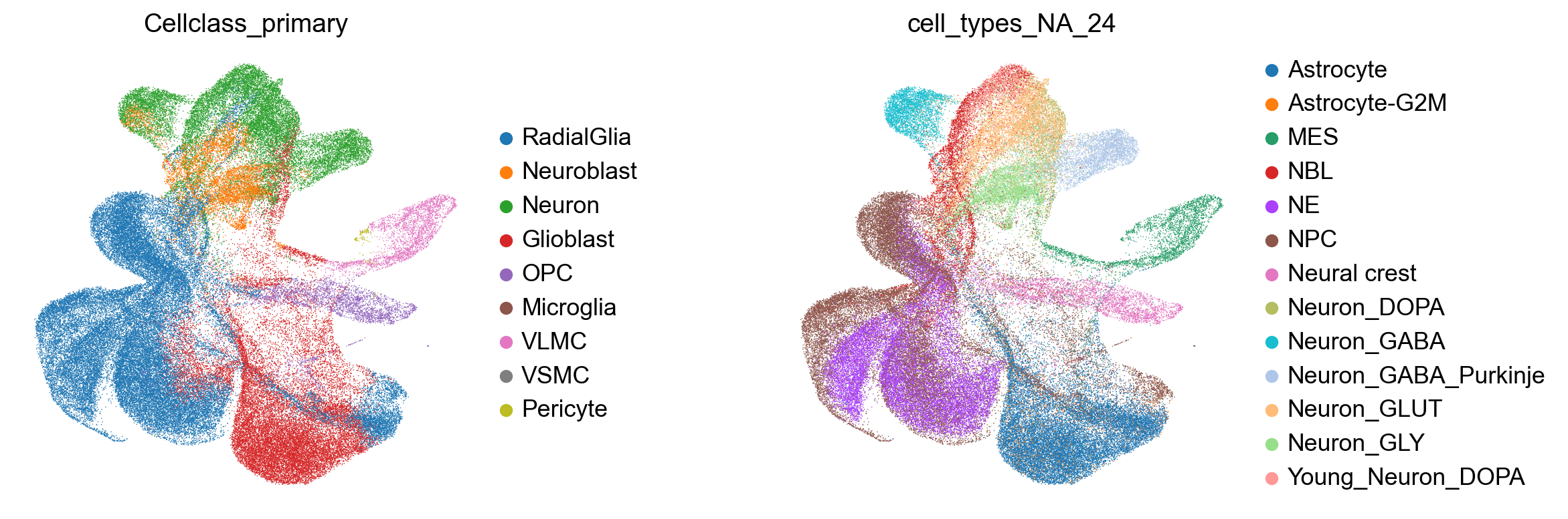
Visualize Results#
Let’s visualize the mapping results to see how well the query data aligns with the reference. For this we would use CellMapper package.
import cellmapper
cmap = cellmapper.CellMapper(query=mapped_adata, reference=adata_ref)
cmap.compute_neighbors(use_rep="X_scpoli", only_yx=False, n_neighbors=50)
cmap.compute_mapping_matrix("hnoca")  # jaccard_square weighting scheme
cmap.map_obs(key="Cellclass", prediction_postfix="primary")  # we transfer Cellclass labels
INFO     Initialized CellMapper with 104452 query cells and 99732 reference cells.
INFO     Using sklearn to compute 50 neighbors.
INFO     Computing mapping matrix using method 'hnoca'.
INFO     Row-normalizing the mapping matrix.
INFO     Mapping categorical data for key 'Cellclass' using one-hot encoding.
INFO     Categorical data mapped and stored in query.obs['Cellclass_primary'].
with plt.rc_context({"figure.figsize": (4, 4.5)}):
    sc.pl.embedding(
        mapped_adata,
        basis="X_umap_scpoli",
        color=["Cellclass_primary", "cell_types_NA_24"],  # let's visualise transferred labels and annotated cell types
        frameon=False,
        ncols=2,
        wspace=0.5,
    )
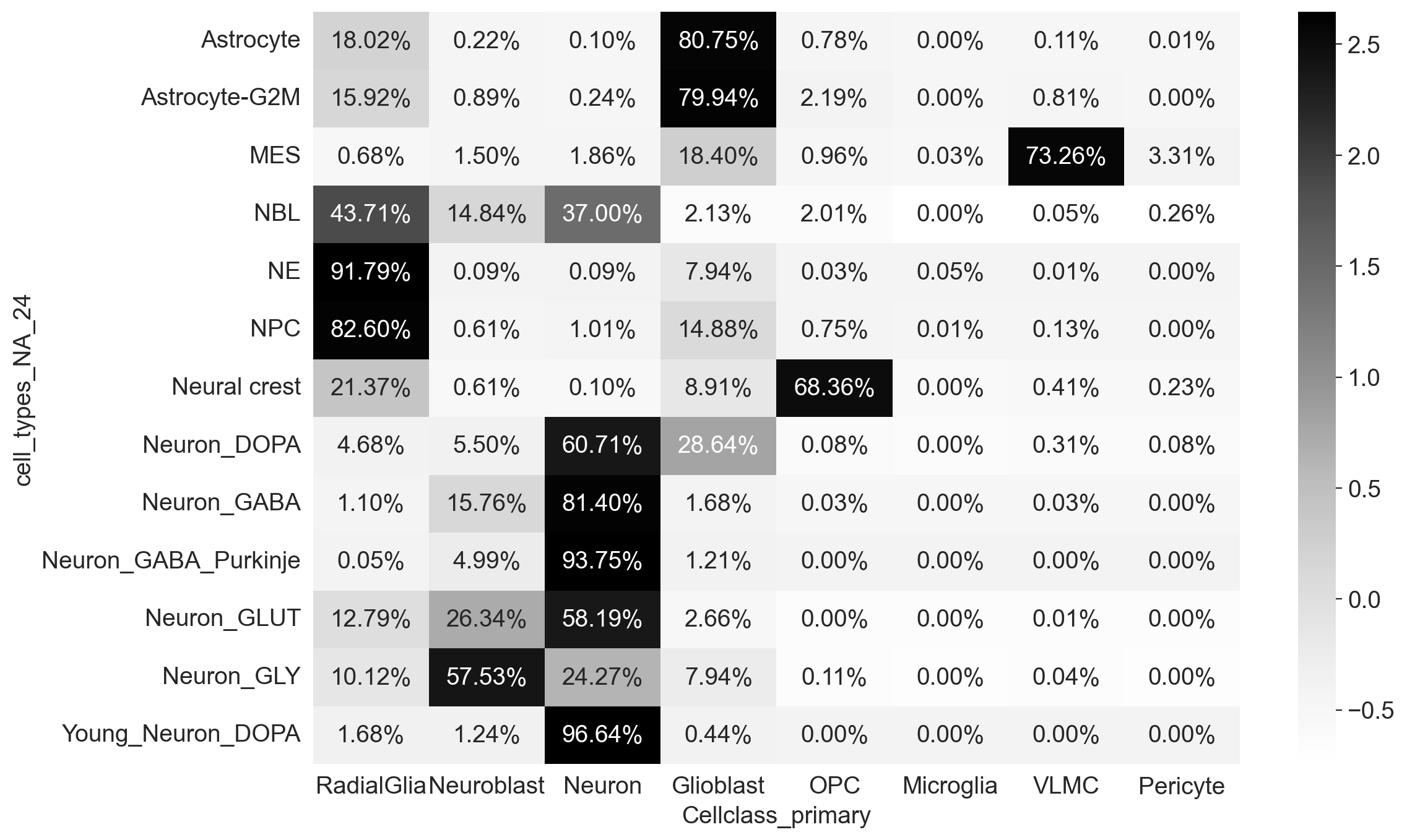
freq_ct_regions = pd.crosstab(mapped_adata.obs.cell_types_NA_24, mapped_adata.obs.Cellclass_primary)
sns.set_style("white")
prop_ct_regions = freq_ct_regions.apply(lambda x: x / np.sum(x), axis=1)
mat = prop_ct_regions.apply(lambda x: (x - np.mean(x)) / np.std(x), axis=1)
with plt.rc_context({"figure.figsize": (12, 8)}):
    svm = sns.heatmap(mat, annot=prop_ct_regions, cmap="Greys", fmt=".2%")
plt.show()
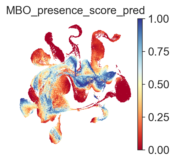
cmap.estimate_presence_score(
    key_added="MBO_presence_score", groupby="sample"
)  # calculate presence score for each cell type in each sample in query data

adata_ref.obs["MBO_presence_score"] = (
    adata_ref.obsm["MBO_presence_score"].max(axis=1) ** 0.5
)  # let's take the maximum presence score for each reference cell across samples
INFO     Presence score across all query cells computed and stored in `reference.obs['MBO_presence_score']`
INFO     Presence scores per group defined in `query.obs['sample']` computed and stored in
         `reference.obsm['MBO_presence_score']`
We can smoothen calculated presence scores.
smap = cellmapper.CellMapper(query=adata_ref)
smap.compute_neighbors(use_rep="X_scpoli", n_neighbors=50)
smap.compute_mapping_matrix("gaussian")
smap.map_obs(key="MBO_presence_score")
INFO     Initialized CellMapper for self-mapping with 99732 cells.
INFO     Using sklearn to compute 50 neighbors.
INFO     Computing mapping matrix using method 'gaussian'.
INFO     Row-normalizing the mapping matrix.
INFO     Mapping numerical data for key 'MBO_presence_score' using direct matrix multiplication.
INFO     Numerical data mapped and stored in query.obs['MBO_presence_score_pred'].
fig, ax = plt.subplots(1, 1, figsize=(3, 3))
sc.pl.embedding(
    adata_ref,
    basis="X_umap_scpoli",
    color=["MBO_presence_score_pred"],
    frameon=False,
    ncols=1,
    wspace=0.5,
    color_map="RdYlBu",
    ax=ax,
    show=False,
    size=2,
)
plt.show()